Affine Registration in 12 lines of code
Yes, you’ve read that correctly! Affine registration can be done in 12 lines of Python using PyTorch. That’s surprising as PyTorch is originally build for deep learning not image registration. But it’s good news for (neuro-)imaging people like me and also a fun toy problem to understand the power of PyTorch. So, if you are interested in neuroimaging and/or deep learning this post will tickle your whistle!
If you are a in a hurry and know what Affine Registration/PyTorch is, simply skip to “The 12 lines” and for the really impatient ones
TL;DR:
- PyTorch is surprisingly effective for image registration due to its
- automatic gradient engine (saving code lines and headaches)
- utility functions F.affine_grid, F.grid_sample and F.interpolate
- GPU support which enables faster compute (on NVIDIA GPU or >2020 Apple Silicon)
- The core of image registration can be coded in 12 lines
- My ~100 lines image registration library installable via
pip install torchregsupports- 2D and 3D images
- GPU computation (speedup!)
- freezing translation, rotation, zoom and/or shear (to do e.g. Rigid Registration)
- multiresolution approaches
- using custom similarity functions/losses and optimizers
- parallel, multimodal and coregistration
What is Affine Registration?
Affine registration is a method which aligns images (e.g. 3D brain-images).
Affine registration applies a combination of translation, rotation, zooming and shearing transformations.
Let’s apply it to two (pointcloudy) fishes to get a visual understanding.
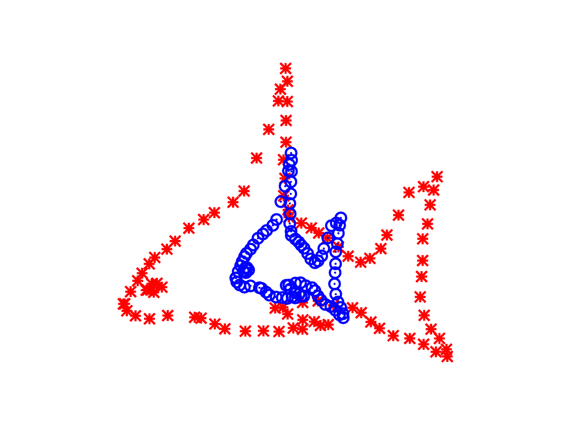
In this example the blue fish - moving image - was aligned (registered) to the red fish - static image - such that each blue point matches the position of its corresponding red point.
Unfortunately, there does not exist a formular that takes two images and returns the desired transformation. But since we can quantify how good the two images are aligned by measuring the mean distances of the respective points we can solve it iteratively - step-by-step. Applied to this problem, an iterative approach does something like this:
- Apply some transformation to moving image
- Calculate distance between points
- If distance > x, apply another transformation to moving image
- Calculate distance between points
- If distance > x, apply another transformation to moving image
- Calculate distance between points
- …
The most naive version of the iterative approach would always apply a random transformation and take a long time until by chance it found a transformation which meets the requirement “distance < x”. As you can see in the GIF, there is a smarter way which smoothly reduces the distance until it meets the requirement. We will get there at the end of “Why PyTorch”!
The transformation can be fully described by an affine matrix \(\mathbf{A}\) (2D: 3x3 matrix, 3D: 4x4 matrix). The \(\mathbf{A}\) matrix encodes:
- translation in its last column
- scale (zoom) on its diagonal
- rotation/shear on all non-diagnoal values of the first two rows/columns
![]()
You might ask “Why encode the transformations in this weird matrix?”. Because we can now transform each coordinate point \(\vec{p}\) by simply multiplying it with this matrix \(\mathbf{A}\).
\[\vec{p}_{\text{moved}} = \mathbf{A} \cdot \vec{p} = \begin{bmatrix} a & b & c\\ d & e & f\\ 0 & 0 & 1\\ \end{bmatrix} \begin{bmatrix} x \\ y \\ 1 \\ \end{bmatrix} = \begin{bmatrix} a \cdot x + b \cdot y + c \\ d \cdot x + e \cdot y + f \\ 1 \\ \end{bmatrix}\]As you can see, we needed to add an extra dimension after \(y\) with a \(\mathrm{1}\) to the 2D point to make it work. In 3D you would have to do the same after the \(z\). Similary, the last row of the affine matrix will always be \(0\) \(0\) … and one \(1\) at the end in 2D and 3D.
Nice, we now introduced all needed concepts to do affine registration in a (naive) iterative fashion! We could write a (slow) program that would randomly stumble towards better aligning affine transformations. Using this starting point we will now march, mumbling the programmers “Make it work, make it pretty, make it fast!”-mantra. Thankfully, PyTorch works fast and is sufficiently pretty such that we will reach the end of the rainbow quite quickly!
Why PyTorch?
PyTorch is primarily used for deep learning and it can be thought of as a NumPy with GPU support (speedup!) since:
- It uses NumPy semantics
import torch
import numpy as np

# Using numpy
zeros  = np.zeros((4, 4))
ones   = np.ones((4, 4))
random = np.random.random((4, 4))
# Using torch
zeros  = torch.zeros(4, 4)
ones   = torch.ones(4, 4)
random = torch.rand(4, 4)- Besides CPU (“normal” processor) it also supports GPU (graphics card) computation, which can be 10-100x faster
import torch

zeros  = torch.zeros(4, 4)
zeros_gpu = zeros.cuda()  # zeros_gpu stored in (NVIDIA) GPU
For our problem (affine registration) it has two more powerful features.
- There exist utility functions which allow you to apply affine transformations to 2D and 3D images!
- PyTorch offers automatic differentiation which is very useful since iterative optimization is much faster when a derivative can be calculated!
To understand the second point we have to answer the following question: What is a gradient?
If you can, try to remember what a derivative is (you probably had to know it during middle school math class).
- The derivative \(\frac{df}{dx}\) of a function \(f(x)\) is its rate of change w.r.t. (with respect to) \(x\).
Let’s make it more concrete and say that \(x\) is an affine matrix and the function \(f\) is the distance of points between two fish images. Wow, what a useful concept for our problem: Now the derivative expresses how much the distance changes w.r.t. the affine matrix. Since \(x\) holds 16 elements (all values of the 4x4 affine matrix) the derivative also contains 16 elements - each simply being the derivative of the distance w.r.t. the respective matrix element. Bravo, this multivariable derivative is the gradient we wanted to understand!
- The gradient \(\nabla\) of a function \(f(x_1, x_2,...)\) is its rate of change w.r.t \(x_1\), \(x_2\),…
The beauty about the gradient is that it always points in the direction (here, affine matrix change) of the maximum increase of the function (here, maximum increase of distance). So, if we want to minimize the distance we just have to change the affine matrix in the opposite direction. Following this direction during our iterative approach, will result in smooth improvement as shown in the GIF.
- Apply some affine to moving image
- Calculate distance between points
- Calculate the gradient of the distance w.r.t affine
- Change affine in descending gradient direction and apply to moving image
- Calculate distance between points
- Calculate the gradient of the distance w.r.t affine
- Change affine in descending gradient direction and apply to moving image
- …
The 12 lines
Now that we know what Affine Registration is and what PyTorch offers us, lets look at the code.
import torch
import torch.nn.functional as F

def affine_registration(moving, static, n_iterations=500, learning_rate=1e-1):
    affine = torch.eye(4)[None, :3]
    affine = torch.nn.Parameter(affine)
    optimizer = torch.optim.SGD([affine], learning_rate)
    for i in range(n_iterations):
        optimizer.zero_grad()
        affine_grid = F.affine_grid(affine, [1, 3, *static.shape])
        moved = F.grid_sample(moving[None, None], affine_grid)
        loss = ((static - moved[0, 0]) ** 2).mean()
        loss.backward()
        optimizer.step()
    return affine.detach()
For people who have used PyTorch for deep learning, the code should look very familiar. It looks like the core component of code which trains a neural net!
Let’s run through it, line by line:
- The function takes a
static(image), amoving(image),n_iterations(number of iterations) and alearning_rate affineis initialized usingtorch.eye(4x4 matrix filled with zeros + ones on diagonal = identity affine)affineis made atorch.nn.Parameterwhich will be optimized if passed to an optimizeroptimizeris initialized using the SGD (Stochastic Gradient Descent) optimizer with the givenlearning_rate- Starting a for-loop which will repeat/iterate lines 6-11 for
n_iterationstimes optimizer.zero_grad()initializes all derivatives (stored in the background) to zeroaffineis transformed into anaffine_grid…- …which is used to apply the affine transformation to the
movingimage lossvalue is the mean squared error (MSE) betweenstaticandmovedimageloss.backward()calculates the derivative/gradient of the loss w.r.t the parameters using the chain rule (loss->moved->affine_grid->affine)optimizer.step()changes theaffinein the opposite of the gradient direction (gradient descent) to minimize the loss- The optimized
affineparameter is converted back to a tensor.detach()and returned
The code deals with (3D) images instead of points now, which is why lines 7-9 need some extra explanation:
First, the MSE in line 7 is doing what the distance between the corresponding red and blue fish points was doing earlier in the post: It measures image alignment. Higher MSEs indicate worse alignment - also called dissimilarity - between moving and static image.
Second, an image can be thought of as a grid of pixels/points.
Applying an affine transformation to each of these pixels - i.e. multiplying its coordinates with the affine matrix, happening in F.affine_grid - works just fine BUT:
You end up with new pixel coordinates which are not placed perfectly on a rectangular grid anymore.
So in 2D each “old” pixel typically ends up somewhere in a 2x2 pixel area of the new image.
The standard approach to deal with this is interpolation which is what F.grid_sample is doing for us in the background.

Application to brain images
After this theoretical fugazi you might think “Talk is cheap, just show me a demo!” so here we go. Using this Colab notebook you can run the whole demo by simply clicking “Runtime” -> “Run all”!
Let’s download two brain images
import nibabel as nib
import urllib.request

def download(url, filepath):
    urllib.request.urlretrieve(url, filepath)

url_stem = 'https://openneuro.org/crn/datasets/ds003835/snapshots/1.0.0/files'
moving_fpath, static_fpath = 'moving.nii.gz', 'static.nii.gz'
download(f'{url_stem}/sub-10:anat:sub-10_T1w.nii.gz', moving_fpath)
download(f'{url_stem}/sub-20:anat:sub-20_T1w.nii.gz', static_fpath)
# Load niftis
moving_nii = nib.load(moving_fpath)
static_nii = nib.load(static_fpath)
and plot them (using .orthoview()) to see how misaligned the brains are
moving_nii.orthoview()static_nii.orthoview()The moving_nii-brain is not as accurately aligned with the crosshairs as the static_nii-brain.
We will fix that by registering moving_nii to static_nii!
Therefore, we have to firstly convert these .nii-files (called “Nifti”) into PyTorch tensors.
# Get numpy arrays out of niftis
moving = nib.as_closest_canonical(moving_nii).get_fdata()
static = nib.as_closest_canonical(static_nii).get_fdata()
# Convert numpy arrays to torch tensors
moving = torch.from_numpy(moving).float()
static = torch.from_numpy(static).float()
And then we can apply our beautiful affine_registration function.
# Reduce resolution to 32³
size = (32, 32, 32)
moving_small = F.interpolate(moving[None, None], size)[0, 0]
static_small = F.interpolate(static[None, None], size)[0, 0]
# Normalize image intensity (minimum is 0 so dividing by maximum is sufficient)
moving_small = moving_small / moving_small.max()
static_small = static_small / static_small.max()
# Do affine registration
optimal_affine = affine_registration(moving_small, static_small)
Oops, I snuck two more operations in there:
- Reducing the masks resolution because
affine_registrationwill be much faster this way - Using
_ / _.max()to normalize image intensities to the value range 0.0-1.0
Finally, we use the optimal_affine to align the moving tensor
affine_grid = F.affine_grid(optimal_affine, [1, 3, *static.shape])
moved = F.grid_sample(moving[None, None], affine_grid)[0, 0]
Did we do everything right? Let’s visualize to check!
moved.orthoview()The moved_nii is accurately aligned to the crosshairs so it worked fine! 🎉
Optionally, we can convert the tensor back to a Nifti which can be saved:
moved_nii = nib.Nifti1Image(moved.cpu().numpy(), static_nii.affine)
moved_nii.to_filename('moved.nii.gz')torchreg: Tiny PyTorch image registration library
Welcome to the advertising bit of this post!
You did not really think I would go through the trouble of explaining you all this stuff, just to share my excitement about short code, did ya?!
I have added a few tweaks and tricks which are missing to make it a “mature” registration tool and ended up with ~100 lines I named torchreg.
torchreg supports 2D and 3D images and can be installed via pip
pip install torchregand provides you with the AffineRegistration class
from torchreg import AffineRegistration

# Load images as torch Tensors
moving = ...
static = ...
# Intialize AffineRegistration
reg = AffineRegistration(is_3d=True)
# Run it!
moved = reg(moving, static)
which supports
- using a multiresolution approach to save compute (per default it runs with 1/4 and then 1/2 of the original resolution for 500 + 100 iterations)
reg = AffineRegistration(scales=(4, 2), iterations=(500, 100))- choosing which operations (translation, rotation, zoom, shear) to optimize
reg = AffineRegistration(with_zoom=False, with_shear=False)- optimization with custom initial parameters
reg = AffineRegistration(zoom=torch.Tensor([1.5, 2., 1.]))- and using custom dissimilarity functions and optimizers
def dice_loss(x1, x2):
    dim = [2, 3, 4] if len(x2.shape) == 5 else [2, 3]
    inter = torch.sum(x1 * x2, dim=dim)
    union = torch.sum(x1 + x2, dim=dim)
    return 1 - (2. * inter / union).mean()

reg = AffineRegistration(dissimilairity_function=dice_loss, optimizer=torch.optim.Adam)
With
moved = reg(moving.cuda(), static.cuda())you can leverage your GPU (if you have a NVIDIA GPU) and speed up the registration.
You can easily access the affine
affine = reg.get_affine()and the four parameters
translation = reg.parameters[0]
rotation = reg.parameters[1]
zoom = reg.parameters[2]
shear = reg.parameters[3]
Thats it with the advertising bit!
Conclusion
I think your conclusions out of this blog post highly depend on your background. Hopefully they look something like this:
- You are a neuroimaging person
- I finally really understand this “Affine Registration” my toolboxes uses
- PyTorch is some neural network stuff. I didn’t fully understand that part but it enables really fast image registration!
- The next time I’ll align Niftis I’ll use torchreg!
- I’ll give the repo a star!
- You are a deep learning person
- I finally kinda understand what PyTorch does in the background of the training loops I always use…
- …but I will play with the Colab notebook and plot/print affine, moved and gradients in the loop to get a feeling for what is happening in the background!
- The word gradient does not scare me anymore!
- If I ever want to apply Affine/Rigid Registration I’ll use torchreg!
- I’ll give the repo a star!
- You are a nerd
- Interesting read, nice comprehensive + short code!
- I’ll give the repo a star because this post entertained me!
- You are a normie
- What is this weird guy talking about?!
One last closing remark: Affine registration in neuroimaging can be made really robust using brainmasks. If you are interested in how to get really accurate masks, take a look into my next blog post (online soon)!